Table of Contents
- Introduction
- Position and Displacement
- Time
- Distance and Average Speed
- Average Velocity
- Instantaneous Velocity and Speed
- Average Acceleration
- Negative Acceleration vs Deceleration
- Instantaneous Acceleration
Introduction
- We begin our study of kinematics by defining the kinematic quantities considering straight line motion in one dimension, referred to as rectilinear motion. This means that the particle that moves is constrained to move along a straight line.
Position and Displacement
-
In order to describe the motion of an object, you must first be able to describe its position, i.e. where it is at any particular time. More precisely, you need to specify its position relative to a convenient reference frame. Earth is often used as a reference frame, and we often describe the position of an object as it relates to stationary objects in that reference frame.
-
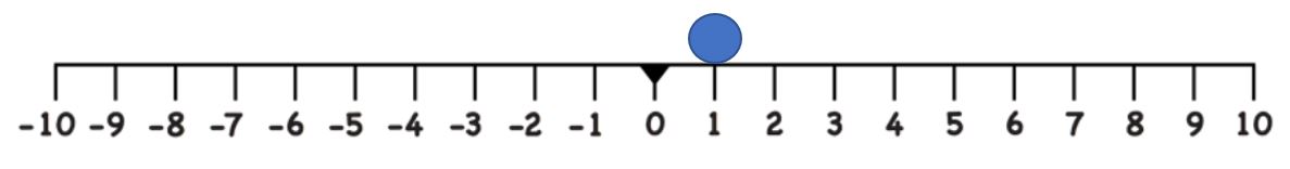
In rectilinear motion, we can simply use a number line (reference frame) to track the motion of an object. In the following example, we say that the position of the object is $x=1$, which corresponds to its coordinate on the number line.
- Displacement is the change in position of an object from its initial position to its final position. It is a vector quantity that describes the shortest distance between the initial position ($x_0$) and final position ($x_f$) of an object. It is denoted by the symbol $\Delta x$.
Displacement
Displacement is the change in position of an object given as:
$\boxed{\Delta{x} = x_f - x_0 }$
where $x_0$ is the initial position and $x_f$ is the final position.
-
Note that the SI unit for displacement is the meter (m).
-
Displacement has a direction as well as a magnitude. The direction is always pointing from the initial position to the final position.
-
In rectilinear motion, it suffices to know the sign of the displacement $\Delta x$ in order to know the direction in which the object is moving. A positive $\Delta x$ means that the object has moved in the direction of increasing $x$. A negative $\Delta x$ means that the object has moved in the direction of decreasing $x$.
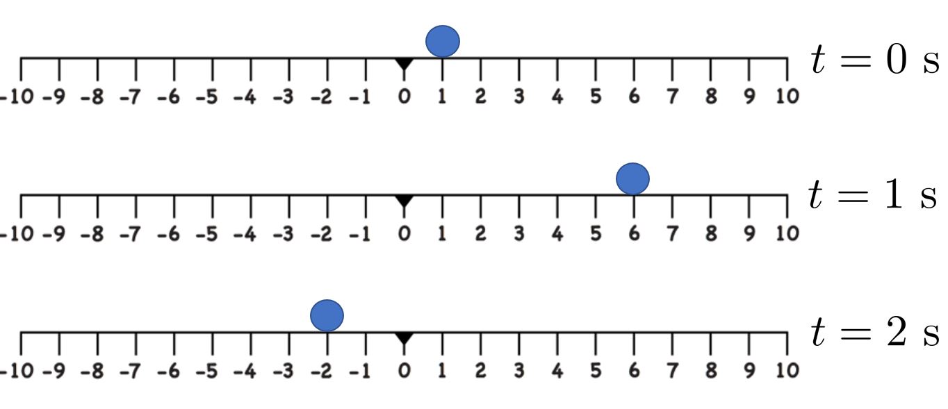
A particle is at $x=1$m when the clock starts. At $t=1$s, it is recorded to be at $x=6$m and at $t=2$s, it is recorded to be at $x=-2$m. Find
(a) the displacement of the particle from $t=0$s to $t=1$s.
(b) the displacement of the particle from $t=0$s to $t=2$s.
(c) the displacement of the particle from $t=1$s to $t=2$s.
Solution (click to expand)
Time
-
Every measurement of time involves measuring a change in some physical quantity. For example, we may be interested in how the position of the Sun in the sky changes with time.
-
Motion occurs when there is a change in the position of an object with respect to time.
-
An important quantity in Kinematics is called the elapsed time $\Delta t$ during which motion occurs. It is the difference between the ending time ($t_f$) and starting time ($t_0$).
$$\boxed{\Delta t = t_f - t_0}$$
- To simplify calculations, we typically start our clock only when motion starts so that $t_0 = 0$ and let $t_f = t$. In this case, $\Delta t = t-0=t$.
Distance and Average Speed
-
Distance or distance travelled is a scalar quantity that describes the magnitude of the path traveled by an object without considering its direction.
-
Average speed is defined as the distance traveled divided by elapsed time.
$$\boxed{\text{Average Speed} = \frac{\text{Distance Travelled}}{\Delta t} }$$
A particle is at $x=1$m when the clock starts. At $t=1$s, it is recorded to be at $x=6$m and at $t=2$s, it is recorded to be at $x=-2$m. Find
(a) the distance travelled and displacement of the particle from $t=0$s to $t=2$s.
(b) the average speed of the particle from $t=0$s to $t=2$s.
Solution (click to expand)
Average Velocity
Average Velocity
The average velocity during an interval of time $\Delta t$ is the ratio of the change in position $\Delta x$ (displacement) to the elasped time $\Delta t$.
$\boxed{\overline{v} = \frac{\Delta x}{\Delta t}}$
-
Note that the above definition indicates that velocity is a vector because displacement $\Delta x$ is a vector. Therefore, it has both a magnitude and a direction. In rectilinear motion, the direction is indicated by the sign. A positive sign means the displacement is in the positive direction, and vice versa.
-
The SI unit for velocity is meters per second or m/s.
-
The average velocity $\overline{v}$ over a time interval $\Delta t$ can be computed as the slope of the secant line joining two points on the position-time ($x$-$t$) graph corresponding to $\Delta t$.

- The average velocity of an object does not tell us anything about its velocity between the starting and ending points.
A particle is at $x=1$m when the clock starts. At $t=1$s, it is recorded to be at $x=6$m and at $t=2$s, it is recorded to be at $x=-2$m. Find
(a) the average speed of the particle from $t=0$s to $t=2$s.
(b) the average velocity of the particle from $t=0$s to $t=2$s.
Solution (click to expand)
-
The above example demonstrates that while the average speed tells us (on average) how fast the object was moving during the elapsed time ($\Delta t$), the average velocity may not always be meaningful for a finite time interval $\Delta t$.
-
Nevertheless, the average velocity is used to defined a more important quantity called the instantaneous velocity.
Instantaneous Velocity and Speed
-
In the above definition of the average velocity $\overline{v}$, imagine we zoom into a small segment of the motion and compute $\overline{v}$. According to the definition, this will simply give us the average velocity over that small $\Delta t$.
-
Now, imagine we make the elapsed time $\Delta t$ so small that we are left with an infinitesimally small time interval. Over such an interval, the average velocity becomes the instantaneous velocity or the velocity at an instant.
-
Instantaneous velocity $v$ is the average velocity at a specific instant in time (or over an infinitesimally small time interval).
Instantaneous Velocity
The instantaneous velocity is a vector quantitiy that gives the speed and direction of an object at a specific instant $t$. Mathematically, it is the limit of the average velocity $\overline{v}$ as the elapsed time $\Delta t$ approaches zero:
$\boxed{v(t) = \lim_{\Delta t \to 0} \frac{\Delta x}{\Delta t} = \frac{dx}{dt} }$
We say that $v(t)$ is the rate of change of position $x$ with respect to time $t$.
-
The instantaneous velocity is typically referred to simply as the velocity.
-
Note that the velocity is a function of time as is evident from the expression $v(t)$.
-
From Calculus, the velocity $\displaystyle v(t)=\frac{dx}{dt}$ is simply the slope (gradient of the tangent) of the $x$-$t$ graph at the instant $t$.

- In the above $x$-$t$ graph, we consider the three time intervals:
$$ \Delta t_1 = t_6 - t_1, \quad \Delta t_2 = t_5 - t_2, \quad \Delta t_3 = t_4 - t_3 $$
- Note that $\Delta t_3 < \Delta t_2 < \Delta t_1$. These time intervals correspond to the following displacements:
$$ \Delta x_1 = x_6 - x_1, \quad \Delta x_2 = x_5 - x_2, \quad \Delta x_3 = x_4 - x_3 $$
- The average velocities corresponding to the three elapsed time intervals are computed as the slope of the secant line joining the starting and end points on the $x$-$t$ graph:
$$\textcolor{red}{\overline{v}_1 = \frac{\Delta x_1}{\Delta t_1}}, \quad \textcolor{teal}{\overline{v}_2 = \frac{\Delta x_2}{\Delta t_2}}, \quad \textcolor{BlueViolet}{\overline{v}_3 = \frac{\Delta x_3}{\Delta t_3}} $$
-
The instantaneous velocity $v(t_0)$ is the slope of the tangent line at $t=t_0$. According to the definition, as $\Delta t \to 0$, the average velocity approaches the instantaneous velocity $v(t_0)$ at $t=t_0$.
-
The above figure demonstrates that the slope of the secant line (average velocity) approaches the slope of the tangent line (instantaneous velocity) as $\Delta t \to 0$ at $t=t_0$ .
Given the $x$-$t$ graph of an object below, find the corresponding velocity-time ($v$-$t$) graph.

Solution (click to expand)

During the time interval between $0$ s and $0.5$ s, the object’s position is moving away from the origin and the position-versus-time curve has a positive slope. At any point along the curve during this time interval, we can find the instantaneous velocity by taking its slope, which is $+1$ m/s.
In the subsequent time interval, between $0.5$ s and $1.0$ s, the position doesn’t change and we see the slope is zero. From $1.0$ s to $2.0$ s, the object is moving back toward the origin and the slope is $−0.5$ m/s. The object has reversed direction and has a negative velocity.
- Instantaneous speed ($s$) is just the magnitude of instantaneous velocity.
$$\boxed{s= |v|}$$
-
For example, suppose a runner at one instant has an instantaneous velocity of $−3.0$ m/s, and if we define the negative direction to the left, then we know the person is running towards the left with a speed of $3.0$ m/s. The velocity contains information on direction, but the speed is just a magnitude.
-
Once again, we typically refer to instantaneous speed simply as speed in subsequent sections.

-
In the above figure, the $x$-$t$ graph, $v$-$t$ graph and $s$-$t$ graph an object are shown.
-
We observe that the $v$-$t$ graph is obtained from the $x$-$t$ graph simply by computing its slope at two segments where the slope is constant i.e. $0$s to $0.25$s and $0.25$s to $0.5$s.
-
The $s$-$t$ graph is obtained from the $v$-$t$ graph by taking only absolute values from the $v$-$t$ graph.
Average Acceleration
- In everyday language, to accelerate means to speed up. The greater the acceleration, the greater the change in velocity over a given time.
Average Acceleration
The average acceleration during an interval of time $\Delta t$ is the ratio of the change in velocity $\Delta v$ to the elasped time $\Delta t$.
$\boxed{\overline{a} = \frac{\Delta v}{\Delta t}}$
-
Since acceleration is velocity in m/s divided by time in s, the SI unit for acceleration is m/s$^2$ (meters per second squared).
-
Note that acceleration changes due to a change in velocity ($\Delta v$) which is a vector quantity. Such a change can be due to either a change in direction or a change in magnitude of $v$. For example, if a car makes a turn at constant speed, there will still be a change in acceleration since direction changes.
-
The average acceleration $\overline{a}$ over a time interval $\Delta t$ can be computed as the slope of the secant line joining two points on the $v$-$t$ graph corresponding to $\Delta t$.

A car accelerates from rest to a velocity of $15.0~$m/s due West in $1.80~$s. What is its average acceleration?
Solution (click to expand)

Negative Acceleration vs Deceleration
-
Deceleration is defined as the process of slowing down (speed decreasing).
-
What can you deduce from a negative average acceleration? Is the object slowing down (decelerating)? Not quite.
-
Negative acceleration $\ne$ deceleration. A negative average acceleration (from $\overline{a} = \frac{\Delta v}{\Delta t}$) means that the change in velocity is also negative. This can mean one of two scenarios from the table below:
- object is travelling in the positive direction and slowing down.
- object is travelling in the negative direction and speeding up.
Table - Sign of acceleration and velocity in different scenarios.
| Scenario | Velocity $v$ | Speed $|v|$ | Acceleration | What It Means |
|---|---|---|---|---|
| (a) | ➕ | Increasing | ➕ | Speeding Up in ➕ direction |
| (b) | ➕ | Decreasing | ➖ | Slowing Down in ➕ direction |
| (c) | ➖ | Decreasing | ➕ | Slowing Down in ➖ direction |
| (d) | ➖ | Increasing | ➖ | Speeding Up in ➖ direction |

-
We realize that if the signs for both acceleration and velocity are the same, then the object is speeding up.
-
Conversely, if the signs for both acceleration and velocity are different, then the object is slowing down.
Instantaneous Acceleration
-
In the above definition of the average acceleration $\overline{a}$, imagine we zoom into a small segment of the motion and compute $\overline{a}$. According to the definition, this will simply give us the average acceleration over that small $\Delta t$.
-
Now, imagine we make the elapsed time $\Delta t$ so small that we are left with an infinitesimally small time interval. Over such an interval, the average acceleration becomes the instantaneous acceleration or the acceleration at an instant.
-
Instantaneous acceleration $a$ is the average acceleration at a specific instant in time (or over an infinitesimally small time interval).
Instantaneous Acceleration
The instantaneous acceleration is the limit of the average acceleration $\overline{a}$ as the elapsed time $\Delta t$ approaches zero:
$\boxed{a(t) = \lim_{\Delta t \to 0} \frac{\Delta v}{\Delta t} = \frac{dv}{dt} }$
We say that $a(t)$ is the rate of change of velocity $v(t)$ with respect to time $t$.
-
The instantaneous acceleration is typically referred to simply as the acceleration.
-
From Calculus, the acceleration $a(t)= \frac{dv}{dt}$ is simply the slope (gradient of the tangent) of the $v$-$t$ graph at the instant $t$.
