Table of Contents
Introduction
Similar to Python lists, we can can also use access NumPy subarrays with the slice notation with the aid of the colon (:) character. The NumPy slicing syntax follows that of the standard Python list.
We begin this section by first importing the NumPy package and creating 3 random arrays using the numpy.random.choice function and seeding the PRNG
so that results are reproducible by the reader.
Example
A 1-D random array.1import numpy as np
2R = np.random.RandomState(32) #set a random seed
3a1 = R.choice(10, size=10, replace=False)
4print(a1)
[9 1 2 8 3 0 4 6 5 7]
Example
A 2-D random array.1a2 = R.choice(3*4, size=(3,4), replace=False)
2print(a2)
[[ 8 10  0  2]
 [ 6  7  1 11]
 [ 4  9  5  3]]
Example
A 3-D random array.1a3 = R.choice(3*4*5, size=(3,4,5), replace=False)
2print(a3)
[[[21  8  7 25  1]
  [53 31 23 44 12]
  [ 3 54 37 51 42]
  [45 14 22 27 34]]

 [[28 57 52 40 17]
  [32  9  2 59 39]
  [33 15 46 43 24]
  [35 58 19 16 41]]

 [[ 4 30  6 49  0]
  [48 47 29 26 56]
  [11 13 38  5 55]
  [36 50 20 10 18]]]
The above random arrays are the same as those used in the previous section on Array Indexing.
Slicing of 1-D Arrays
The NumPy array slicing syntax follows that of the standard Python list.
Syntax
Slicing a 1-D array.1array[start=0:stop=size of array:step=1]
| Parameter | Required? | Default Value | Description |
|---|---|---|---|
start |
❌ No | 0 | An integer number specifying at which position to start the slicing. |
stop |
❌ No | Size of array. | An integer number specifying at which position to end the slicing (output excludes endpoint). |
step |
❌ No | 1 | An integer number specifying the step of the slicing. |
Python and NumPy both use half-open intervals: the start index is included while the stop index is not.
Example
Printing a 1-D array. The following are all equivalent.1print(a1[0:a1.size:1]) # 10 is the size
2print(a1[::])
3print(a1[:])
4print(a1)
[9 1 2 8 3 0 4 6 5 7]
[9 1 2 8 3 0 4 6 5 7]
[9 1 2 8 3 0 4 6 5 7]
[9 1 2 8 3 0 4 6 5 7]
We see that the same a1 array is printed whether one colon (:) or two colons (::) are enclosed within the square brackets (with no numbers specified).
Slicing with Positive Indices
The following shows the positive index of each element of the 1-D array a1.
| Positive Index | 0 | 1 | 2 | 3 | 4 | 5 | 6 | 7 | 8 | 9 |
|---|---|---|---|---|---|---|---|---|---|---|
| Element | 9 | 1 | 2 | 8 | 3 | 0 | 4 | 6 | 5 | 7 |
Example
Slicing a 1-D array (positive indices).1a1[5:] # all elements after index 5
array([0, 4, 6, 5, 7])
Example
Slicing a 1-D array (positive indices).1a1[4:7] # subarray
array([3, 0, 4])
Example
Slicing a 1-D array (positive indices).1a1[::3] # # step size of 3
array([9, 8, 4, 7])
Example
Slicing a 1-D array (positive indices).1a1[:7:2] # every other element, stop at index=7
array([9, 2, 3, 4])
Example
Slicing a 1-D array (positive indices).1a1[3::2] # every other element, starting at index 3
array([8, 0, 6, 7])
Slicing with Mixed Indices
Mixed indices refer to a combination of both positive and negative indices. The following shows the negative index of each element of the 1-D array a1. The last element has an index of -1, the second last element has an index of -2 and so on.
| Negative Index | -10 | -9 | -8 | -7 | -6 | -5 | -4 | -3 | -2 | -1 |
|---|---|---|---|---|---|---|---|---|---|---|
| Element | 9 | 1 | 2 | 8 | 3 | 0 | 4 | 6 | 5 | 7 |
Example
Slicing a 1-D array (mixed indices).1a1[::-1] # all elements, reversed.
array([7, 5, 6, 4, 0, 3, 8, 2, 1, 9])
Example
Slicing a 1-D array (mixed indices).1a1[5:1:-1] # reversed from index 5 to index 2
array([0, 3, 8, 2])
| Positive Index | 0 | 1 | 2 | 3 | 4 | 5 | 6 | 7 | 8 | 9 |
|---|---|---|---|---|---|---|---|---|---|---|
| Element | 9 | 1 | 2 | 8 | 3 | 0 | 4 | 6 | 5 | 7 |
Example
Slicing a 1-D array (mixed indices).1a1[-3:-8:-2] # reversed (every other) from index -3 to index -7
array([6, 0, 8])
| Negative Index | -10 | -9 | -8 | -7 | -6 | -5 | -4 | -3 | -2 | -1 |
|---|---|---|---|---|---|---|---|---|---|---|
| Element | 9 | 1 | 2 | 8 | 3 | 0 | 4 | 6 | 5 | 7 |
ADVERTISEMENT
Slicing of 2-D Arrays.
Syntax
Slicing of 2-D arrays.1array[start=0:stop=n1:step=1, start=0:stop=n2:step=1]
where n1 is the size of the first dimension (number of rows) and n2 is the size of the second dimension (number of columns).
| Parameter | Required? | Default Value | Description |
|---|---|---|---|
start |
❌ No | 0 | An integer number specifying at which position to start the slicing. |
stop |
❌ No | Size of dimension. | An integer number specifying at which position to end the slicing (output excludes endpoint). |
step |
❌ No | 1 | An integer number specifying the step of the slicing. |
Example
Printing a 2-D array. The following are all equivalent.1print(a2[0:a2.shape[0]:1,0:a2.shape[1]:1])
2print(a2[:,:])
3print(a2[::,::])
4print(a2[0:a2.shape[0]:1,:])
5print(a2)
[[ 8 10  0  2]
 [ 6  7  1 11]
 [ 4  9  5  3]]

[[ 8 10  0  2]
 [ 6  7  1 11]
 [ 4  9  5  3]]

[[ 8 10  0  2]
 [ 6  7  1 11]
 [ 4  9  5  3]]

[[ 8 10  0  2]
 [ 6  7  1 11]
 [ 4  9  5  3]]

[[ 8 10  0  2]
 [ 6  7  1 11]
 [ 4  9  5  3]]
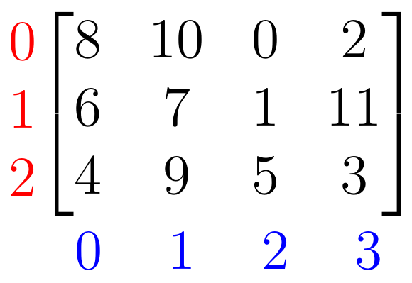
In a 2-D NumPy array, we can access elements using a comma-separated tuple of 2 indices: (row index, column index). For example, for the a2 array, the first index (red) represents the row index (top to bottom) and second index (blue) represents the column index (left to right).
Example
Slicing a 2-D array.1a2[:2, :] # 1st two rows
array([[ 8, 10,  0,  2],
       [ 6,  7,  1, 11]])
Example
Slicing a 2-D array.1a2[: , :3] # 1st 3 colummns
array([[ 8, 10,  0],
       [ 6,  7,  1],
       [ 4,  9,  5]])
Example
Slicing a 2-D array.1a2[:2, :3] # 1st two rows, 1st three columns
array([[ 8, 10,  0],
       [ 6,  7,  1]])
Example
Slicing a 2-D array (every other row).1a2[::2 , :] # every other row
array([[ 8, 10,  0,  2],
       [ 4,  9,  5,  3]])
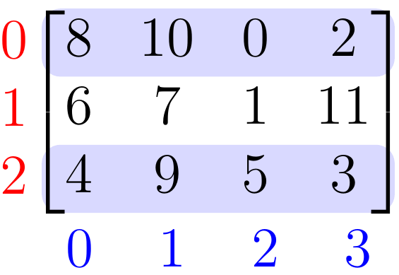
Since row access is quite common in NumPy, there is a shortcut to slicing rows. We can simply insert an array of row indices within the square brackets.
Example
Slicing a 2-D array (every other row).1a2[[0,2]] # every other row
array([[ 8, 10,  0,  2],
       [ 4,  9,  5,  3]])
To access the rows of a 2-D array, we can simply insert an array of row indices within the square brackets: a2[row_indices].
Alternatively, the following code works as well.
Example
Slicing a 2-D array (every other row).1a2[np.arange(3)[::2]] # every other row
array([[ 8, 10,  0,  2],
       [ 4,  9,  5,  3]])
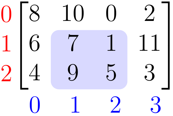
Example
Slicing a 2-D array.1a2[1:, 1:3] #subarray
array([[7, 1],
       [9, 5]])
Example
Reversing rows of a 2-D array.1a2[::-1 , :] # rows reversed
array([[ 4,  9,  5,  3],
       [ 6,  7,  1, 11],
       [ 8, 10,  0,  2]])
Example
Reversing columns of a 2-D array.1a2[: , ::-1] # columns reversed
array([[ 2,  0, 10,  8],
       [11,  1,  7,  6],
       [ 3,  5,  9,  4]])
ADVERTISEMENT
Slicing of 3-D Arrays.
Syntax
Slicing of 3-D arrays.1array[start=0:stop=n1:step=1, start=0:stop=n2:step=1, start=0:stop=n3:step=1]
| Parameter | Required? | Default Value | Description |
|---|---|---|---|
start |
❌ No | 0 | An integer number specifying at which position to start the slicing. |
stop |
❌ No | Size of dimension. | An integer number specifying at which position to end the slicing (output excludes endpoint). |
step |
❌ No | 1 | An integer number specifying the step of the slicing. |
where the stop index is given by:
stop index |
Code | Description |
|---|---|---|
n1 |
numpy.ndarray.shape[0] |
Number of frames. |
n2 |
numpy.ndarray.shape[1] |
Number of rows. |
n3 |
numpy.ndarray.shape[2] |
Number of columns. |
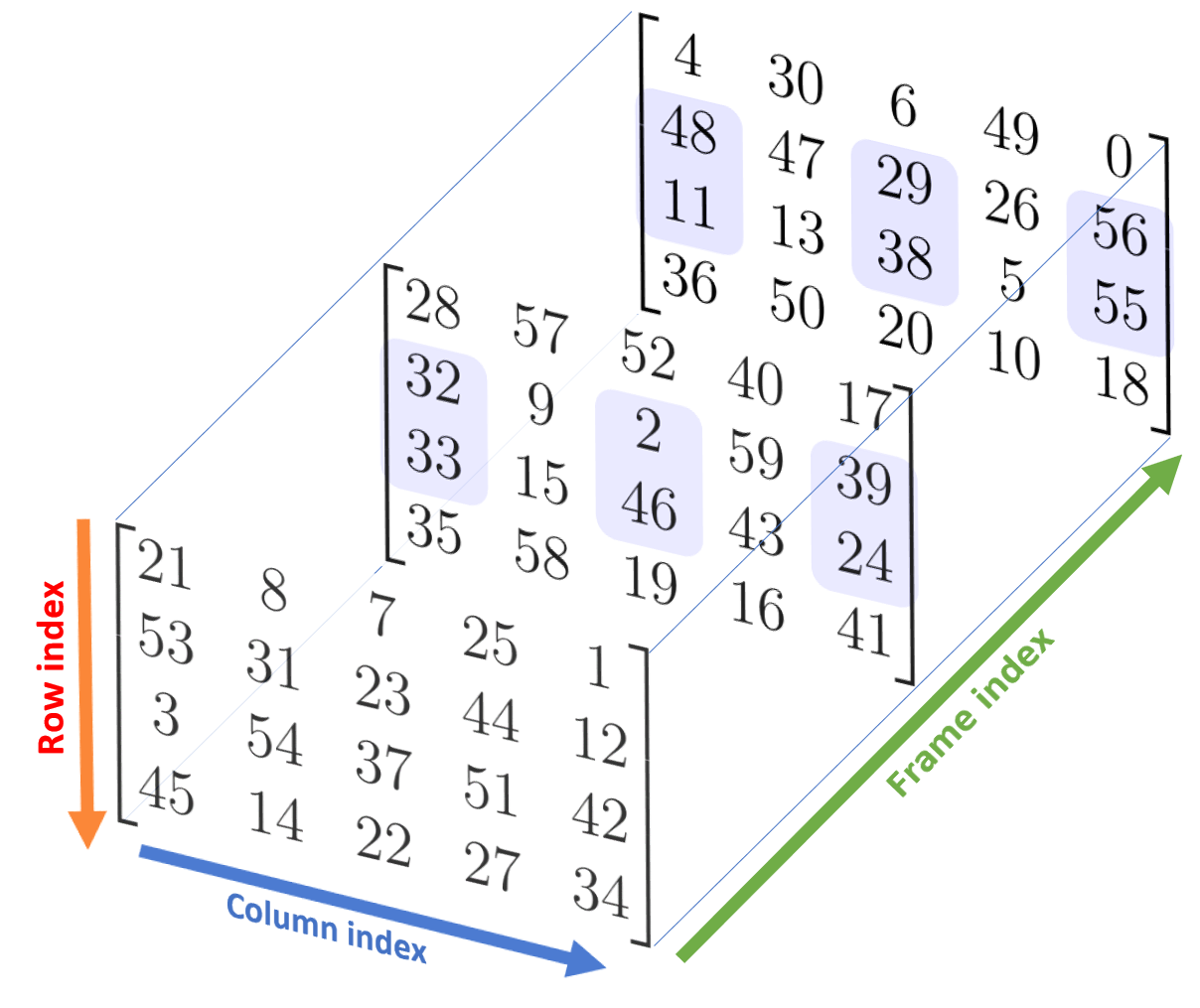
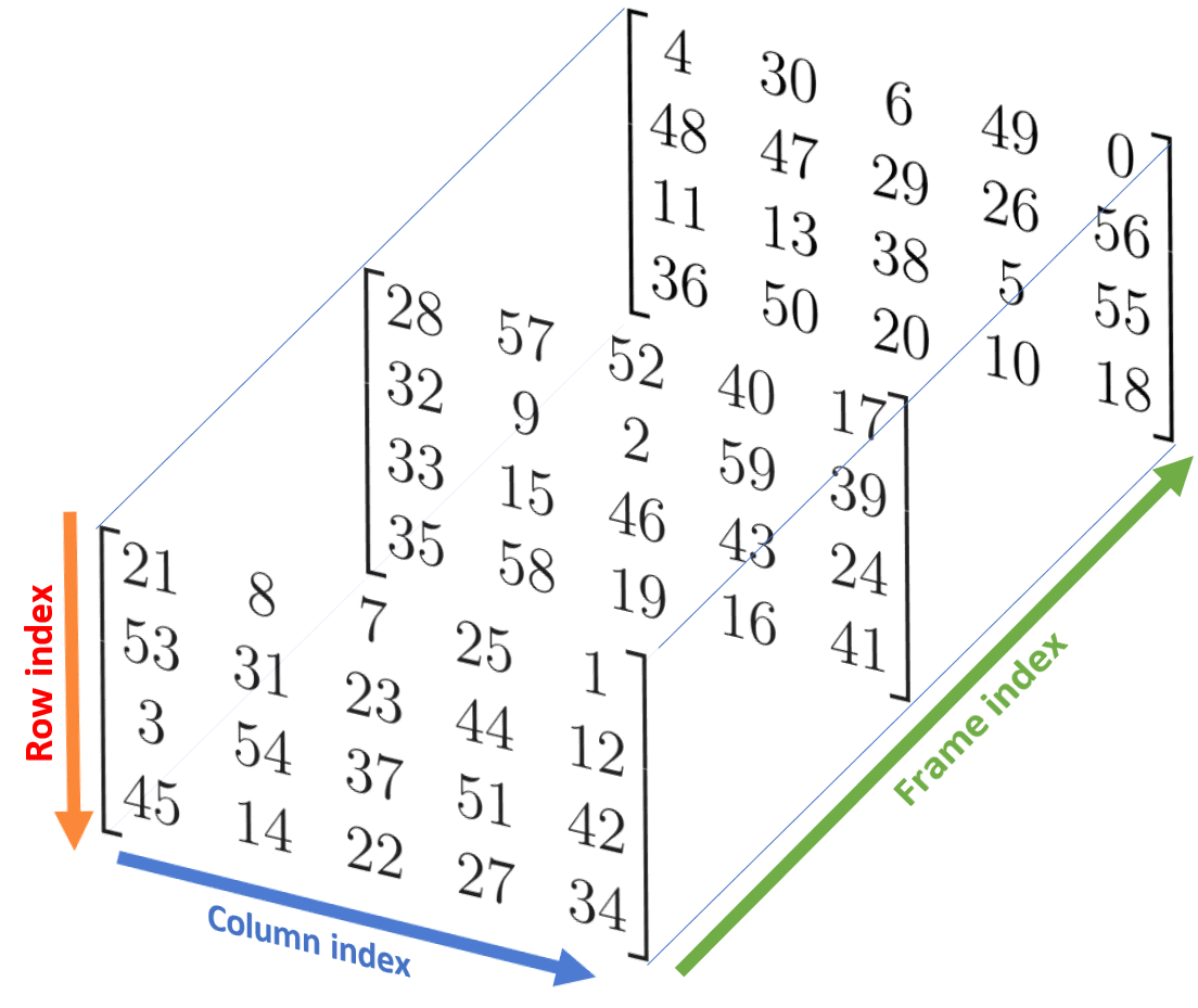
In a 3-D NumPy array, we can access elements using a comma-separated tuple of 3 indices: (frame index, row index, column index). For example, for the a3 array, the first index (green) indicates the frame index, the second index (red) represents the row index (top to bottom) and third index (blue) represents the column index (left to right). The ouput is typically printed frame by frame.
Example
Printing a 3-D array. The following are all equivalent.1print(a3[0:a3.shape[0]:1, 0:a3.shape[1]:1, 0:a3.shape[2]:1])
2print(a3[:,:,:])
3print(a3[::,::,::])
4print(a3[0:a3.shape[0]:1,:,:])
5print(a3[0:a3.shape[0]:1,0:a3.shape[1]:1,:])
6print(a3[:,0:a3.shape[1]:1,:])
7print(a3[:,:,0:a3.shape[2]:1])
8print(a3)
[[[21  8  7 25  1]
  [53 31 23 44 12]
  [ 3 54 37 51 42]
  [45 14 22 27 34]]

[[28 57 52 40 17]
  [32  9  2 59 39]
  [33 15 46 43 24]
  [35 58 19 16 41]]

[[ 4 30  6 49  0]
  [48 47 29 26 56]
  [11 13 38  5 55]
  [36 50 20 10 18]]]
Note that the above list is not exhaustive. Other configurations are possible.
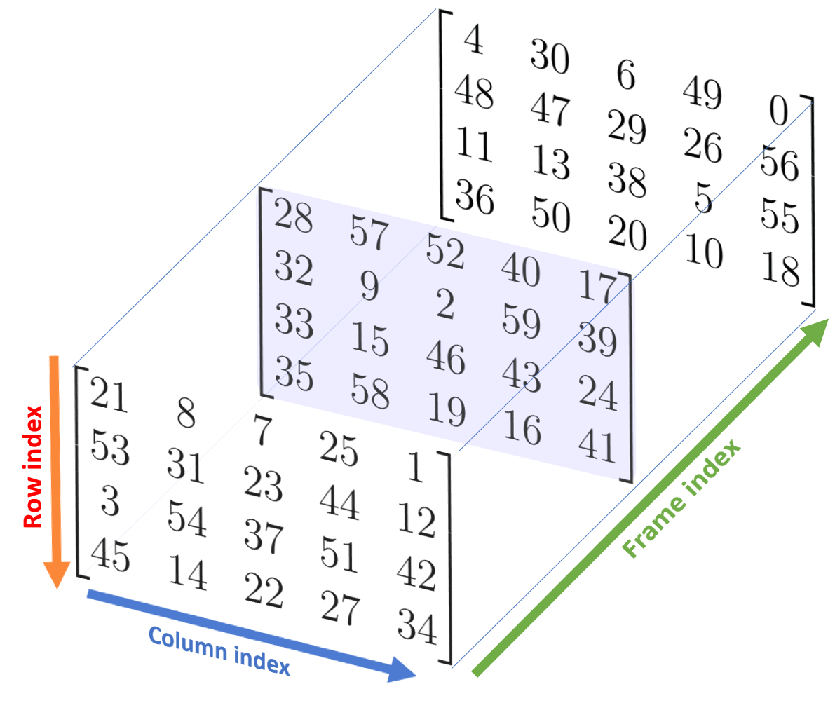
Example
Slicing a 3-D array.1a3[1,:,:] # second frame
array([[28, 57, 52, 40, 17],
       [32,  9,  2, 59, 39],
       [33, 15, 46, 43, 24],
       [35, 58, 19, 16, 41]])
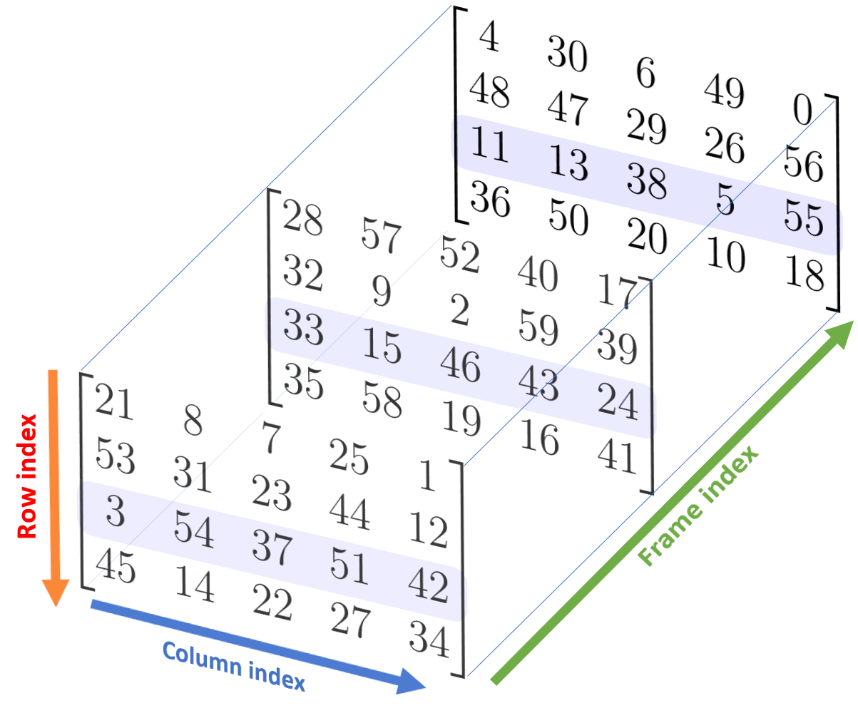
Example
Slicing a 3-D array.1a3[:,2,:] # third row
array([[ 3, 54, 37, 51, 42],
       [33, 15, 46, 43, 24],
       [11, 13, 38,  5, 55]])
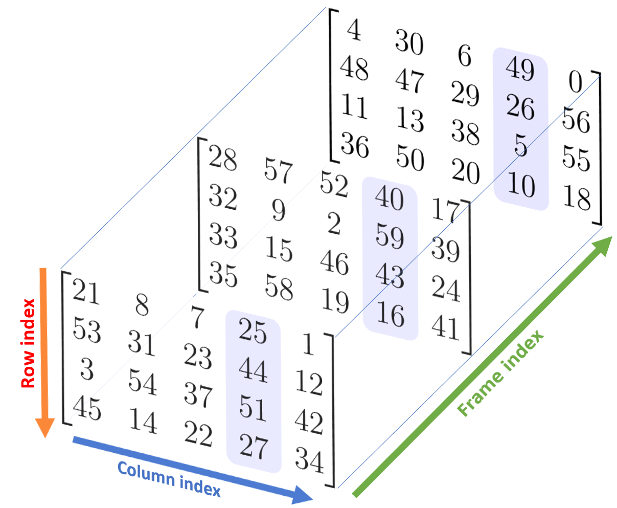
Example
Slicing a 3-D array.1a3[:,:,3] # 4th column
array([[25, 44, 51, 27],
       [40, 59, 43, 16],
       [49, 26,  5, 10]])
Example
Slicing a 3-D array.1a3[1:,1:3,::2] # subarray
array([[[32,  2, 39],
        [33, 46, 24]],

       [[48, 29, 56],
        [11, 38, 55]]])