Table of Contents
Introduction
NumPy provides the trigonometric ufuncs np.sin(x), np.cos(x) and np.tan(x) that take values in radians and produce the corresponding $\sin x$, $\cos x$ and $\tan x$ values. In this article, we will examine their usage and demonstrate how we can use the ufuncs to realize various transformations such as shifting, stretching and reflection.
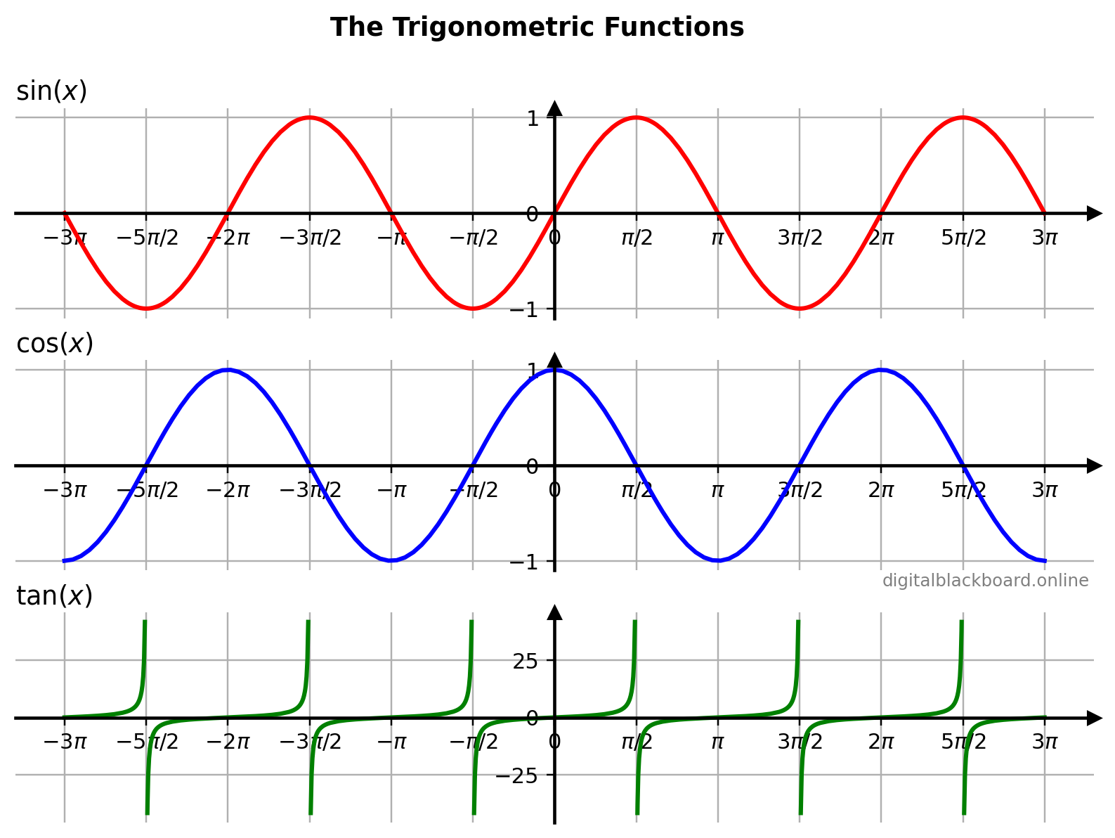
The following table lists the 3 basic trigonometric ufuncs available in NumPy.
| Function | Ufunc | Input x |
Domain of Function | Description |
|---|---|---|---|---|
| $\sin x$ | np.sin(x) |
radians | $-\infty \leq x \leq \infty$ | Sine function |
| $\cos x$ | np.cos(x) |
radians | $-\infty \leq x \leq \infty$ | Cosine function |
| $\tan x$ | np.tan(x) |
radians | $\displaystyle \left\{ x \in \mathbb{R} | x \ne (2n + 1)\frac{\pi}{2}, n\in \mathbb{Z} \right\}$ | Tangent function |
$\pi~ \text{radians} = 180^{\circ}$
Computing the Trigonometric Ufuncs
We first define the domain using the np.linspace function. Note that np.pi generates the mathematical constant $\pi$. The theta array consists of 5 values.
$$\theta = \left[0 \quad \frac{\pi}{2} \quad \pi \quad \frac{3\pi}{2} \quad 2\pi \right] $$
Example
Computing the trigonometric functions.1import numpy as np
2theta = np.linspace(0, 2*np.pi, 5)
3print(theta) # theta values
4print(np.around(np.sin(theta),3)) # sin
5print(np.around(np.cos(theta),3)) # cos
6print(np.around(np.tan(theta),3)) # tan
[0. 1.57079633 3.14159265 4.71238898 6.28318531]

[ 0.  1.  0. -1. -0.]

[ 1.  0. -1. -0.  1.]

[ 0.00000000e+00  1.63312394e+16 -0.00000000e+00  5.44374645e+15
-0.00000000e+00]
Note that $\tan(\theta)$ is undefined at $\displaystyle\theta = \frac{\pi}{2}$ and $\displaystyle\theta = \frac{3\pi}{2}$. This explains the infinitely large values at these two points.
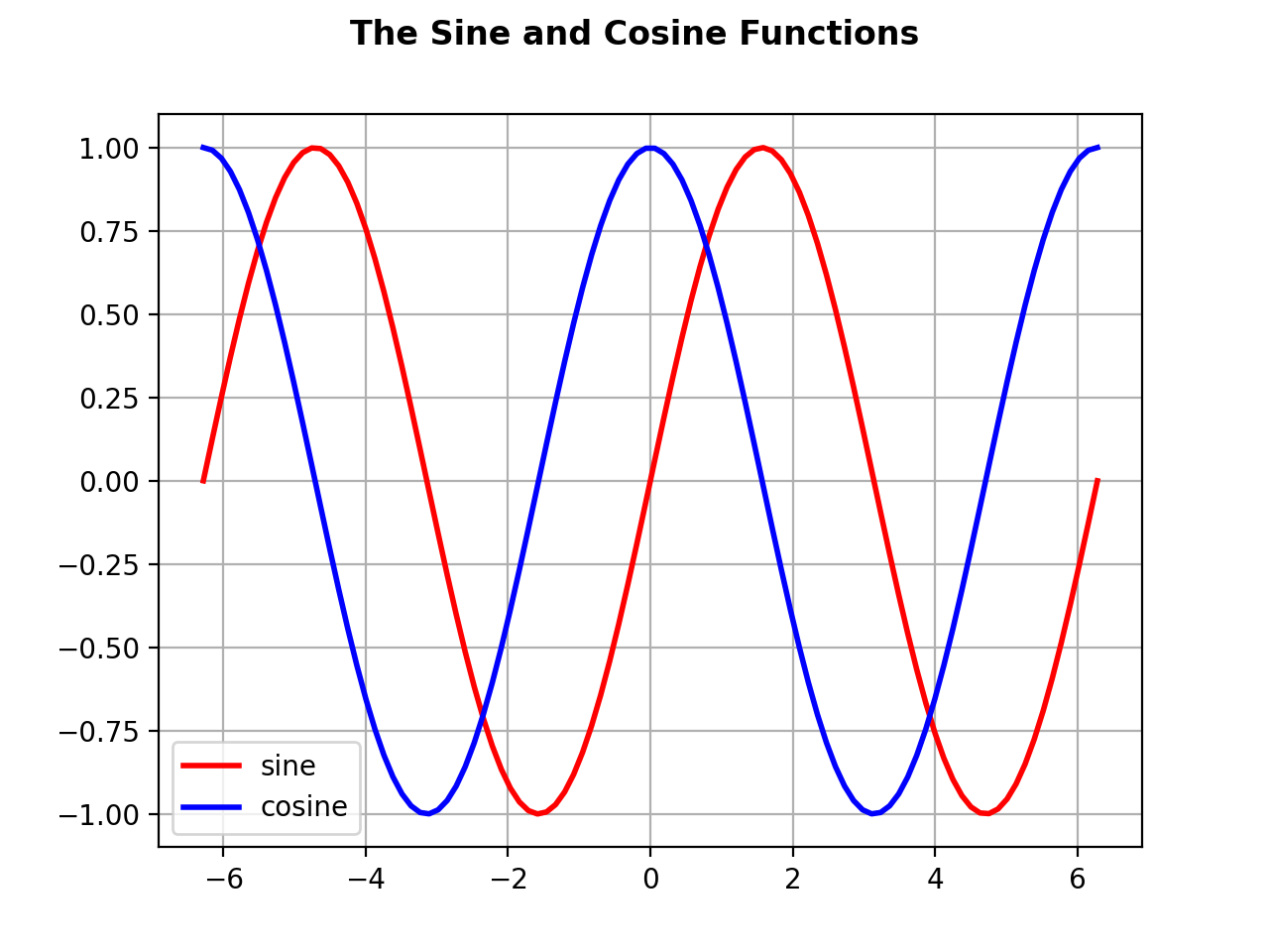
The $\sin x$ and $\cos x$ functions are plotted below using the Matplotlib library which we will discuss in detail in a separate course. For now, we will restrict ourselves to basic plotting commands.
1import matplotlib.pyplot as plt
2plt.figure(0)
3plt.plot(x, np.sin(x), 'r-',   linewidth=2, label="sine")
4plt.plot(x, np.cos(x), 'b-',   linewidth=2, label="cosine")
5plt.grid(True)
6plt.suptitle('The Sine and Cosine Functions', fontweight = 'bold')
7plt.legend(loc="lower left")
It is possible to generate professional-looking plots using the Matplotlib library. In the following figure, we plot the 3 trigonometric functions in 3 separate subplots using radians in the abscissa.
ADVERTISEMENT
Transformations
In this section, we will discuss some basic transformations of the trigonometric functions using the NumPy ufuncs. These include shifting, scaling and reflection.
Shifting in the $x$-direction
- If the argument $x$ of a function $f$ is replaced by $x-h$, then the graph of the new function $y = f(x-h)$ is the graph of $f$ shifted horizontally right by $h$ units.
- If the argument $x$ of a function $f$ is replaced by $x+h$, then the graph of the new function $y = f(x+h)$ is the graph of $f$ shifted horizontally left by $h$ units.
Example
Shifting in the $x$-direction.1x = np.linspace(-2*np.pi, 2*np.pi, 100) # domain
2np.sin(x-np.pi/2) # shifted right
3np.sin(x)
4np.sin(x+np.pi/2) # shifted left
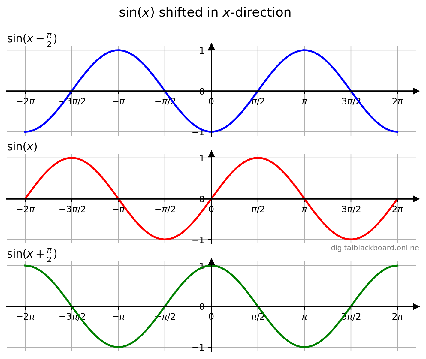
- The second subplot displays the original graph of $\sin x$ defined within the domain $-2\pi \leq x \leq 2\pi$.
- The first subplot displays the graph of $\sin (x-\frac{\pi}{2})$ which is the graph of $\sin x$ being shifted by $\frac{\pi}{2}$ units to the right.
- The second subplot displays the graph of $\sin (x+\frac{\pi}{2})$ which is the graph of $\sin x$ being shifted by $\frac{\pi}{2}$ units to the left.
Shifting in the $y$-direction
- The graph of $f(x)+k$ is the graph of $f(x)$ shifted vertically up by $k$ units.
- The graph of $f(x)-k$ is the graph of $f(x)$ shifted vertically down by $k$ units.
Example
Shifting in the $y$-direction.1x = np.linspace(-2*np.pi, 2*np.pi, 100) # domain
2np.sin(x)+1 # shifted up
3np.sin(x)
4np.sin(x)-1 # shifted down
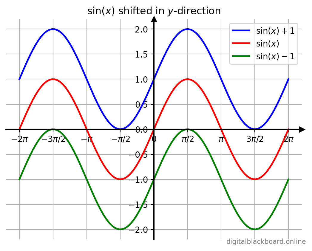
- The line in red displays the original graph of $\sin x$ defined within the domain $-2\pi \leq x \leq 2\pi$.
- The line in blue displays the graph of $\sin(x)+1$ which is the graph of $\sin x$ being shifted vertically up by $1$ unit.
- The line in green displays the graph of $\sin(x)-1$ which is the graph of $\sin x$ being shifted vertically down by $1$ unit.
Scaling in the $x$-direction
- A horizontal compression results if $a>1$.
- A horizontal stretch results if $0< a < 1 $.
Example
Scaling in the $x$-direction.1x = np.linspace(-2*np.pi, 2*np.pi, 100) # domain
2np.sin(0.5*x) # a=0.5, scaled in x by factor 2
3np.sin(x)
4np.sin(2*x) # a=2, scaled in x by factor 1/2
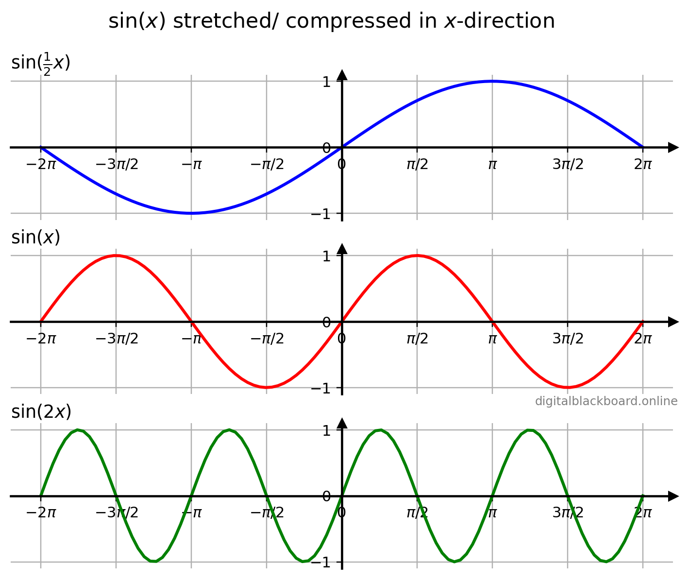
- The second subplot (line in red) displays the original graph of $\sin x$ defined within the domain $-2\pi \leq x \leq 2\pi$.
- The first subplot (line in blue) displays the graph of $\sin(\frac{1}{2}x)$ which is the graph of $\sin x$ being stretched by a factor of $2$ in the $x$-direction.
- The third subplot (line in green) displays the graph of $\sin(2x)$ which is the graph of $\sin x$ being compressed by a factor of $\frac{1}{2}$ in the $x$-direction.
ADVERTISEMENT
Scaling in the $y$-direction
- A vertical stretch results if $a>1$.
- A vertical compression results if $0< a < 1 $.
Example
Scaling in the $y$-direction.1x = np.linspace(-2*np.pi, 2*np.pi, 100) # domain
22*np.sin(x) # scaled in y by factor 2
3np.sin(x)
40.5*np.sin(x) # scaled in y by factor 1/2
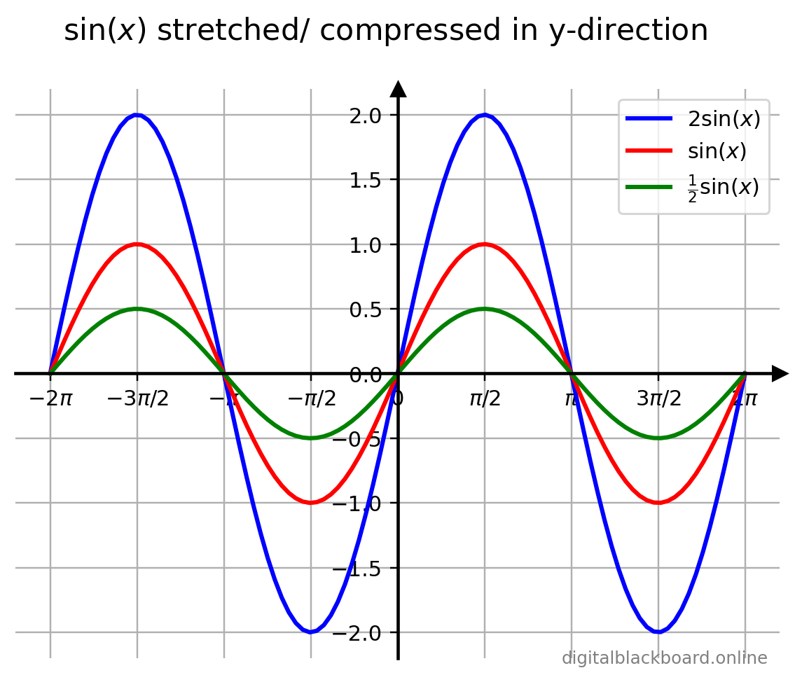
- The line in red displays the original graph of $\sin x$ defined within the domain $-2\pi \leq x \leq 2\pi$.
- The line in blue displays the graph of $2\sin(x)$ which is the graph of $\sin x$ being stretched by a factor of $2$ in the $y$-direction.
- The line in green displays the graph of $\frac{1}{2}\sin(x)$ which is the graph of $\sin x$ being compressed by a factor of $\frac{1}{2}$ in the $y$-direction.
Reflection about the $x$-axis
When a function $y = f(x)$ is multiplied by $-1$, the graph of the new function $y = -f(x)$ is the reflection about the $x$-axis of the graph of $y = f(x)$.
Example
Reflection about the $x$-axis.1x = np.linspace(-2*np.pi, 2*np.pi, 100) # domain
2np.sin(x)
3-np.sin(x) # reflected about the x-axis
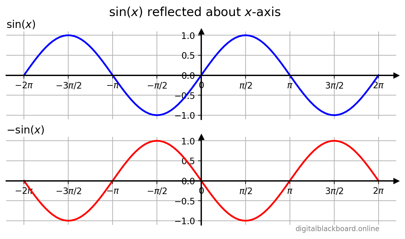
- The first subplot (line in blue) displays the original graph of $\sin x$ defined within the domain $-2\pi \leq x \leq 2\pi$.
- The second subplot (line in red) displays the graph of $-\sin(x)$ which is the graph of $\sin x$ reflected about the $x$-axis.
Reflection about the $y$-axis
If the argument $x$ of a function $y = f(x)$ is multiplied by $-1$, then the graph of the new function $y = f(-x)$ is the reflection about the $y$-axis of the graph of $y = f(x)$.
Example
Reflection about the $y$-axis.1x = np.linspace(-2*np.pi, 2*np.pi, 100) # domain
2np.sin(x)
3np.sin(-x) # reflected about the y-axis
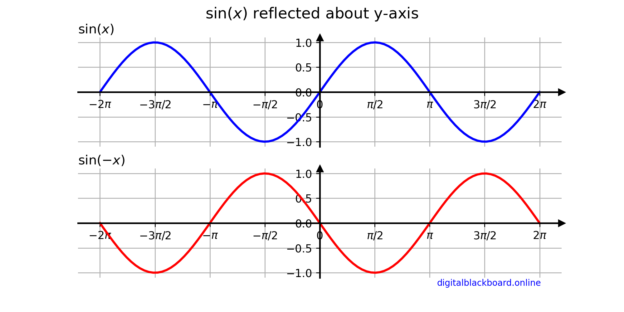
- The first subplot (line in blue) displays the original graph of $\sin x$ defined within the domain $-2\pi \leq x \leq 2\pi$.
- The second subplot (line in red) displays the graph of $-\sin(x)$ which is the graph of $\sin x$ reflected about the $x$-axis.
ADVERTISEMENT
Combining Transformations
It is possible to perform the basic transformations one after another to arrive at more complicated compound transformations. Although the order in which transformations are performed may be immaterial, we recommend using the following order for consistency:
- Reflection.
- Scaling.
- Shifting.
Example
Plot the graph of $\sin (-2x+\pi)$ by performing the relevant transformations.We first note that $$\sin (-2x+\pi) = \sin\left[-2(x- \frac{\pi}{2} )\right]$$
Factor out the coefficient of $x$ in the argument of the trigonometric function before applying the transformations.
1x = np.linspace(-2*np.pi, 2*np.pi, 100) # domain
2np.sin(-x) # Step 1
3np.sin(-2x) # Step 2
4np.sin(-2x+np.pi) # Step 3
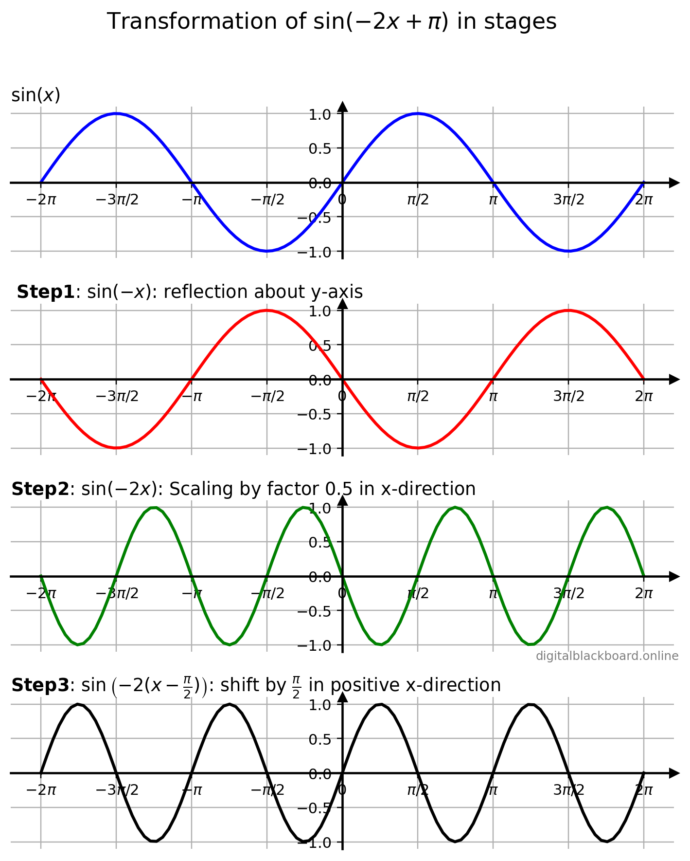
- Step 1: Reflect the graph of $\sin x$ about the $x$-axis to obtain $\sin (-x)$.
- Step 2: Compress the graph of $\sin (-x)$ horizontally by a factor of $0.5$ to obtain $\sin (-2x)$.
- Step 3: Shift the graph of $\sin (-2x)$ horizontally by $\frac{\pi}{2}$ radians to obtain $\sin \left(-2(x-\frac{\pi}{2}) \right)$.
In practice, however, there is no need to perform the transformations in stages. We can just plot np.sin(-2x+np.pi) to obtain the final graph.